What does 'optimal' optimise? The cost function unpacked.

SMART SEWERS· PART 2 OF 6

Asset Management   ·   19 May 2026   ·   Pasi Pajula

Part 1 established that the decision space for a sewer rehabilitation programme is unenumerable. The follow-up question is sharper: what are we optimising for? Any optimisation result is only as good as the objective function — and "minimise lifecycle cost" sounds straightforward until you write out what cost actually contains.

Five components of cost

A defensible cost function for a sewer network needs at least these five terms.

Capex. Rehabilitation and renewal spend — lining, point repairs, open-cut renewal, coordinated street works. For the benchmark utility (~50,000 inhabitants, ~400 km of sewers), a 0.5–1.0 %-per-year rehabilitation pace at 1,000–1,500 € / m of pipe runs to roughly 40–120 M € over a 20-year horizon. The most visible and politically contested item — usually the single largest line, but not larger than the other four combined.

Operational cost. Three distinct opex lines that capex-only optimisation doesn’t see.

(1) Pumping and treating infiltration and inflow. A network where I/I equals 30 % of dry-weather flow sends roughly 30 % more water to the treatment plant than the population produces — and every cubic metre carries roughly 0.25–0.45 € in treatment and pumping at Finnish 2024–26 unit costs. For the benchmark utility this compounds to roughly 4–8 M € over a 20-year horizon.

(2) Planned preventive maintenance. Scheduled sewer cleaning and jetting of sediment-prone reaches, force-main and manhole inspections, pump-station preventive servicing (motor checks, impeller wear, electrical), flow-monitoring and telemetry upkeep. Routine and recurring on a maintenance schedule, not event-triggered: typically 200–800 k€/year for the same utility, or 4–16 M € over 20 years.

(3) Reactive maintenance. Blockage clearing, root cutting, complaint-driven CCTV, and the small spot repairs that don’t qualify as planned rehabilitation. Event-triggered rather than scheduled: typically 150–600 k€/year, or 3–12 M € over 20 years.

Combined operational cost: roughly 11–36 M € over 20 years — material at the budget table, and invisible to a single-objective capex optimiser.

Failure and damage cost. Property damage from sewer surcharges and backflows, traffic disruption from collapses, regulator-driven remediation orders, environmental enforcement. Episodic but heavy-tailed. For the benchmark utility, the expected value over 20 years is roughly 5–15 M € (1–3 major events per year at 100–500 k € per event for repair + damage + remediation), but the 95th-percentile outcome can reach 30–50 M € — a single catastrophic event (major collapse, regulator order, contaminant release) can singly exceed a decade of planned capex. In Finland we do not have this high extreme costs due to the fact that the penalties/sanctions are not so high compared to UK, for example.

Service-level cost. Customer complaints, overflow frequency, interruption hours. Direct financial line items — compensation under SLAs, complaint-handling overhead, regulatory penalties — run roughly 1–4 M € over 20 years for the benchmark utility (Finland is less penalty-heavy than UK, so figures sit at the low end of European benchmarks). The smallest line in pure € terms, but tracked separately by customers, councils, and the regulator because it’s also a political variable.

Environmental cost. Three sub-items, all with carbon or shadow pricing.

Combined-sewer overflows into watercourses at Finnish regulator-implied shadow prices of ~0.5–5 € / m³.

Embodied carbon in rehabilitation works — 5–20 t CO₂ per 100 m of pipe lined or replaced — at a carbon shadow of ~100 € / tCO₂.

Direct process emissions, primarily N₂O from disrupted nitrification. Finnish WWTPs measure emission factors ranging from near 0 % during warm periods to ~1.8 % of influent nitrogen during cold periods (HSY’s Viikinmäki plant alone emits ~134 t N₂O / year, ~86 % of its total GHG output). For the benchmark utility this scales to ~2–5 M € over 20 years at GWP 273 (IPCC AR6) and a 100 €/tCO₂ shadow.

Combined environmental cost: ~4–25 M € over 20 years. The weight on this term is increasing fast in regulator decisions and in ESG reporting.

Ballpark magnitudes side by side

Cost component	Typical 20-year range (mid-sized Finnish utility)
Capex (rehabilitation & renewal)	40–120 M €
Operational (I/I + planned + reactive)	11–36 M €
Failure & damage (expected; heavy upper tail)	5–15 M € (P95 up to 50 M €)
Service-level (financial line items only)	1–4 M €
Environmental (CSO + embodied carbon + process N₂O)	4–25 M €

Capex is the largest single line, but the other four combined can match or exceed it — and minimising capex alone pushes the rest up. Any one of them can swallow the savings if ignored. The trade-offs aren’t translatable into a single euro-equivalent without making a value judgment.

A note on the I/I — N₂O chain. The same infiltration and inflow that drives the operational line above also drives a large share of the environmental line. Cold I/I water (often <4 °C during Finnish snowmelt) slows biological nitrification, and incomplete nitrification is the dominant source of N₂O — a greenhouse gas with 273× the global-warming potential of CO₂. Reducing I/I therefore generates a triple payoff: lower treatment + pumping cost, lower failure risk from hydraulic overloading, and lower process emissions. Capex-only optimisation sees none of these. Year-to-year emissions swing significantly with snowmelt intensity — that uncertainty is exactly the kind Part 3 will fold into the Monte Carlo simulation.

What’s not in the table. The five components above are decision-relevant costs — the ones that change between candidate rehabilitation programmes. They sit on top of a layer of fixed and overhead costs — management, office buildings, fleet, IT, billing, customer service — that for a typical Finnish multi-utility run roughly 1.5–2.5 M €/year combined. After allocation between water supply and sewerage (most utilities use revenue share, putting roughly 30–40 % on the sewer side), the sewer system carries another ~10–18 M € over 20 years. Real cost, real budget line — but approximately constant across rehabilitation plans, so they don’t enter the optimisation trade-off. The optimiser picks between alternatives; fixed costs are the floor every alternative sits on.

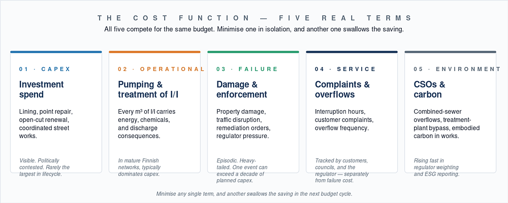
Figure 1. The five real cost terms a sewer rehabilitation programme has to navigate. Minimising any one alone leaves the other four to compound.

The Pareto frontier

This is the structural reason optimisation in sewer asset management is increasingly multi-objective. You cannot minimise five things at once; you can only describe how each candidate programme positions you on the trade-off surface.

The Pareto frontier is the set of candidate programmes for which no single component can be improved without making another worse. Single-objective optimisers find one point — and almost always the wrong one, because the weights are hidden in the model. Multi-objective optimisers find the frontier and hand the political choice (cost vs. risk vs. service vs. environment) back to the people who should make it: the utility board and the elected officials, not the engineering algorithm (Marzouk & Omar 2013).

What each dot represents. Each blue dot on the front is a single, complete 20-year renovation programme — a full decision specifying which action (replace, line, point-repair, defer) and timing to assign to each of the network’s ~30,000 individual pipes. One dot, tens of thousands of asset-level decisions inside it. The optimisation searches through the 10^420000 decision space introduced in Part 1 (typically via evolutionary or metaheuristic algorithms — NSGA-II is the standard reference) and crystallises out the programmes where no objective can be improved without worsening another. Those non-dominated programmes form the front; everything else is dominated and falls below it. Part 3 will then add a Monte Carlo wrapper inside each programme, sampling each pipe’s uncertain inputs to put error bars on the dot itself.

How are the dots generated? The Pareto front isn’t drawn by hand — it’s the output of a multi-objective evolutionary algorithm (NSGA-II is the standard reference). The procedure mimics natural selection: start with a population of a few hundred randomly-generated candidate programmes; score each one on every objective (cost, residual risk, condition, environmental); “reproduce” the best by combining and slightly mutating them to produce the next generation; repeat for several hundred generations. A typical run evaluates 50,000 to 500,000 candidate programmes before the front stabilises — overnight on a workstation, or a few hours on cloud infrastructure. Each evaluation is a full 20-year simulation of all ~30,000 pipes, so the optimisation chews through hundreds of millions of pipe-year calculations. The dots you see at the end are the non-dominated programmes that survived the final generation.

Where does the existing expert plan sit? A manually-crafted engineering know-how programme — drafted by the operators who have spent fifteen or twenty years with this network — can be plotted onto exactly the same axes as the algorithmic candidates. If the expert plan sits on the Pareto front, it’s already non-dominated for the objectives chosen: strong, quantitative validation of operational judgment that the boardroom rarely gets to see expressed in numbers. If it sits inside the front (dominated), there’s at least one algorithmic alternative that does better on every objective simultaneously, by a quantifiable margin — and the conversation moves from “trust me” to “here’s exactly what we’d gain, and where.” Either way, the comparison is on the same methodology and the same cost function. Not algorithm-versus-intuition rhetoric, but two programmes evaluated on a common scale.

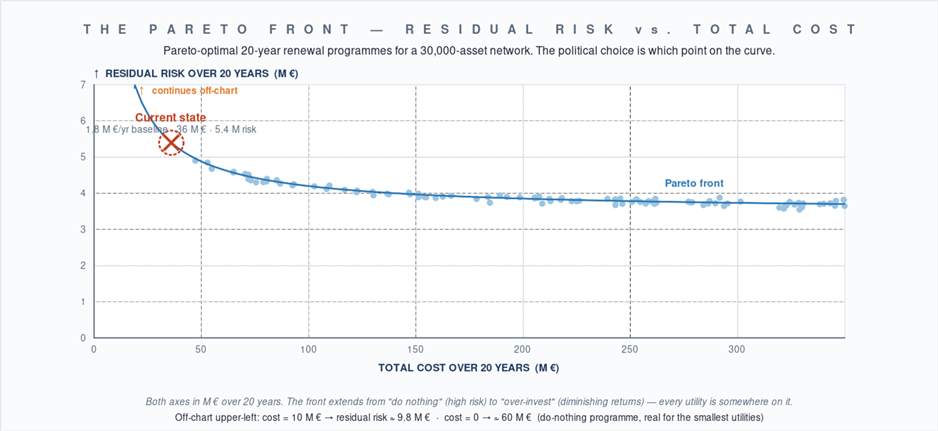
Figure 2a. Pareto-optimal 20-year renewal programmes for a 30,000-asset network. Each point is one full programme — a complete action-and-timing decision for every pipe in the network — not a single pipe. Cost on the X-axis, residual risk on the Y-axis. The current state sits on the front; the political choice is which point on the curve to occupy.

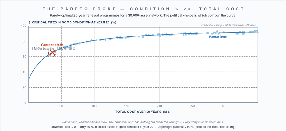
Figure 2b. The same Pareto front re-expressed against condition: % of critical pipes in good condition at the end of the 20-year horizon. Higher is better.

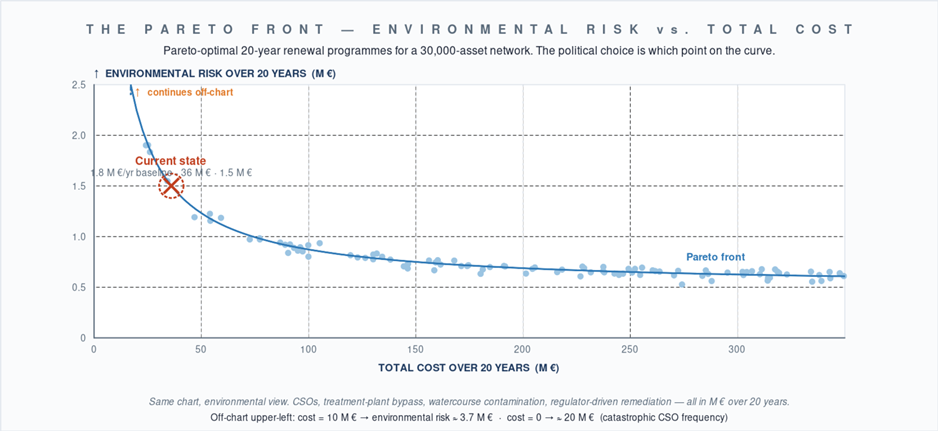
Figure 2c.. The same Pareto front re-expressed against environmental risk: expected CSO volume to watercourses over the 20-year horizon. Lower is better.

Criticality weights the inputs

Before optimisation runs, individual segments need criticality weights. A 600 mm trunk under a hospital is not the same asset as a 100 mm tail under farmland. The cost function structure is identical; the failure-cost coefficients are not. This is where deterministic deterioration models meet network-graph analysis — and it's the input where domain knowledge matters most.

Three takeaways

01 · Cost is plural. A defensible objective function has at least five terms; minimising capex alone is structurally misleading.

02 · The Pareto frontier replaces the single answer. The right question is "which point on the frontier," not "what is the optimum."

03 · Criticality is where domain knowledge lives. Network shape, hospital catchments, watercourse proximity, traffic exposure — all distort the cost function in ways generic tools cannot capture.

NEXT IN THE SERIES

Part 3 — epistemic uncertainty. Monte Carlo simulation and how to put confidence bounds on the optimum.

Further reading

• Marzouk, M. & Omar, M. (2013). Multi-objective optimisation algorithm for sewer network rehabilitation. Structure and Infrastructure Engineering 9(11).

• Tscheikner-Gratl, F. et al. (2016). Sewer asset management under data scarcity. Water Asset Management International 12(2).

• Halfawy, M.R., Dridi, L. & Baker, S. (2008). Integrated decision support system for optimal renewal planning of sewer networks. J. Computing in Civil Engineering 22(6).

  
  

Now in pilot. We are selecting Water utilities for the first deployments of the asset-management optimisation module — built on the US-EPA 10-step procedure and the methods discussed in this series. If you operate a network where the techniques in this post could be used, contact pasi.pajula@preventos.fi.

—

The optimisation methods in this series rely on integrated, data-quality-scored network condition data. Preventos Hero already provides that backbone in daily production use across Finnish water utilities.