Error bars on the optimum: Monte Carlo and the risk profile.
- Pasi Pajula
- May 26
- 4 min read

SMART SEWERS · PART 3 OF 6
Asset Management · 26 May 2026 · Pasi Pajula
Part 2 ended with the Pareto frontier as the structural answer to multi-objective optimisation. Part 3 takes the next step: the frontier itself is uncertain. Every input that feeds the cost function is a distribution, not a number — and that has direct consequences for how an "optimal plan" should be presented to a utility board.
Inputs are distributions, not numbers
Pipe remaining useful life is not 47 years. It is a distribution — material, soil chemistry, installation quality, traffic loading, and a hundred other factors give a spread that, for typical Finnish sewer cohorts, runs from roughly 25 to 90 years with a long upper tail. Annual failure rate is similar: heavy-tailed, log-normal-ish, with most segments stable and a small minority responsible for most events. Repair cost per incident spans an order of magnitude depending on depth, traffic management, and discovery timing. I/I rate varies between catchments by factors of three or more.
Each of these distributions describes the spread of values across the relevant population — across the network’s pipe inventory for RUL and failure rate, across repair events for incident cost, across catchments for I/I. The deterministic optimiser replaces each population with its mean and proceeds as if every pipe, event, and catchment carried that single value. Monte Carlo, in contrast, samples the full distribution at every step of the simulation: pipe by pipe, event by event, catchment by catchment.
A deterministic optimiser takes the mean — or worse, a "professional estimate" — of each input and produces a single optimal programme. The output looks confident. It is not. The confidence bounds are invisible because they were assumed away at the input stage.

Figure 1. Every input to a sewer optimisation model has spread. A deterministic optimiser uses only the dashed lines (the means). Monte Carlo samples the full curves.
Monte Carlo simulation in 30 seconds
The fix is not exotic. One Monte Carlo run is one internally-consistent 20-year future for the whole network. For that run, every pipe gets its own sampled remaining useful life and its own sampled failure rate, every catchment its own sampled I/I, every repair event its own sampled cost — tens of thousands of random draws stitched into one coherent future. Simulate the network’s 20-year trajectory under that future; record the total lifecycle cost, the service-level disruption, the failure count. Then start over with a fresh set of draws, and repeat 5,000 or 10,000 times.
Five thousand can sound small until you notice that each run already aggregates over tens of thousands of pipes — the law of large numbers does most of the within-run work, and the 5,000 figure is what nails down the bigger structural uncertainty. The output is no longer a single number — it is the full distribution of what that programme might deliver across plausible futures.
Run this once for the deterministic optimum, and you discover something uncomfortable: the actual P5–P95 confidence interval on its lifecycle cost is often 20 to 40 percent wide. The "optimal" plan saves a single-digit percentage over the next-best plan in expected value, but its 95th-percentile downside is materially worse. The next-best plan, run through the same simulator, may be more robust.
The output is a band, not a point
This is the practical shift in deliverable. The right answer to a utility board is not "the optimum costs €X over 20 years" — it is "the optimum carries an expected cost of €X, a 90 percent confidence interval of €Y to €Z, and a 95th-percentile worst case of €W." The robustness of the plan becomes a quantifiable property. Two plans with the same expected cost can have very different risk profiles, and the choice between them is — again, as in Part 2 — a political question that the algorithm should not pre-empt.

Figure 2. 5,000 internally-consistent 20-year futures for the same candidate programme. Each tally is one whole-network future, not a per-pipe trial. The deterministic point estimate sits inside a P5–P95 band that is 20–40% wide. The deliverable is the band, not the point.
The same Monte Carlo machinery feeds back into the Pareto frontier from Part 2. Each point on the frontier becomes a small cloud rather than a single coordinate. A defensible plan presentation shows the frontier as a band, not a curve.
Aleatoric vs. epistemic
One distinction worth naming. Aleatoric uncertainty is the inherent randomness — even with perfect knowledge of every pipe, repair costs would still vary. Epistemic uncertainty is what we don't know about the inputs themselves — the deterioration model parameters, the failure-cost coefficients. Monte Carlo handles both, but they behave differently: aleatoric is irreducible; epistemic can be narrowed by better data collection. Treating them separately tells you where to invest in measurement.
Three takeaways
01 · Point estimates are misleading. A single optimal cost number has invisible error bars that are usually wider than the savings it claims.
02 · Monte Carlo gives a risk profile. Sample the inputs, simulate the futures, report the distribution. The right deliverable is a confidence band, not a number.
03 · Robustness becomes quantifiable. Two plans with the same expected cost can have very different 95th-percentile downsides. Choose deliberately.
NEXT IN THE SERIES
Part 4 — external coordination. How the street-renewal programme, district-heating schedule, and telecom rollouts move the optimum by 20–40 percent.
Further reading
Hastings, N.A.J. (2009). Physical Asset Management. Springer. — Monte Carlo treatment for infrastructure life-cycle.
Egger, C. et al. (2013). Sewer deterioration modeling: a review. Water Science & Technology 67(10).
Tscheikner-Gratl, F. et al. (2019). Sewer asset management — state of the art and research needs. Urban Water Journal.
Now in pilot. We are selecting water utilities for the first deployments of the asset-management optimisation module — built on the US-EPA 10-step procedure and the methods discussed in this series. If you operate a network where the techniques in this post could used, contact pasi.pajula@preventos.fi.
—
The optimisation methods in this series rely on integrated, data-quality-scored network condition data. Preventos Hero already provides that backbone in daily production use across Finnish water utilities.